Assalamualaikum Warrahmatullahi wabarakatuh. I’m Raihan Syifa, and in this post, I’d like to present the results of my CFD heat transfer simulation performed in SimScale. This project focuses on a U‑tube heat exchanger with a steel shell and two separate flow regions at 100 °C and 80 °C, respectively. Below, I’ll walk you through the key aspects of the simulation, from the overall setup to the final convergence plots and what they signify about the heat exchanger’s performance.
A. Visualization of Heat Flow
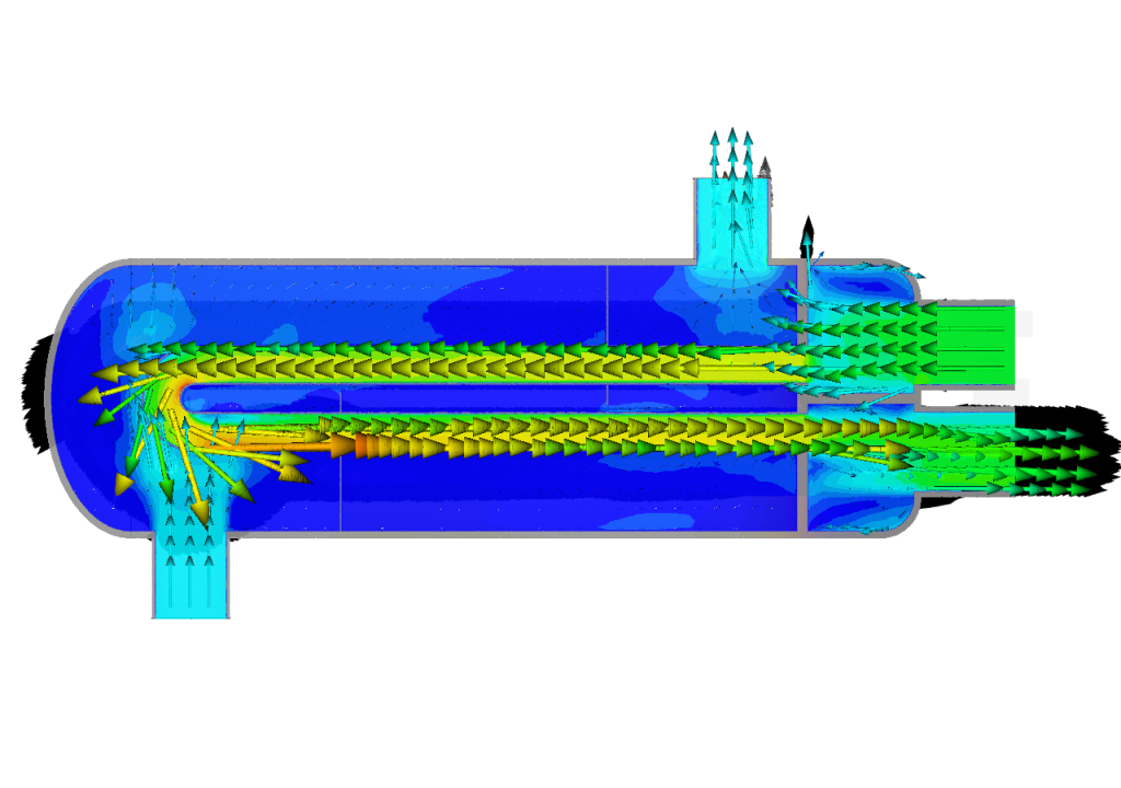
One of the most insightful outputs is the heat flow and velocity field inside the heat exchanger:
- Velocity Arrows:
- The arrows indicate how fluid enters, circulates through the U‑tubes, and exits.
- Areas with higher velocity often appear in brighter colors (green or yellow), especially near inlets and inside the narrower tubes.
- Lower velocity or recirculation zones might be visible in the shell around the tubes, where the flow slows down and mixes more thoroughly.
- Temperature Distribution:
- You can observe a clear gradient between the hot and cold fluid streams.
- The steel walls also show a temperature gradient, with higher temperatures on the side contacting the 100 °C fluid and lower temperatures near the 80 °C fluid.
- This visual confirms that heat is indeed transferring across the metal from the hotter to the cooler fluid.
B. Inlet Convergence Plot
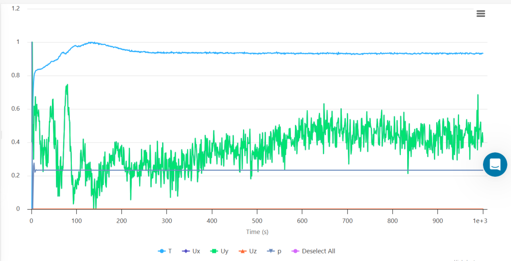
In the second image, the plot (likely in green) tracks one or more quantities—such as velocity or temperature—monitored at the inlet over time or iteration steps.
- Early Oscillations: At the beginning of the simulation, you see larger fluctuations as the solution field (flow + temperature) develops from the initial guess.
- Stabilizing Phase: After some iterations (or seconds, in a transient simulation), the fluctuations diminish, and the monitored variable settles around a near-constant value.
- Sign of Convergence: This leveling off indicates that the flow and temperature at the inlet boundary are no longer changing significantly, a strong indication that the simulation is converging.
C. Outlet Convergence Plot
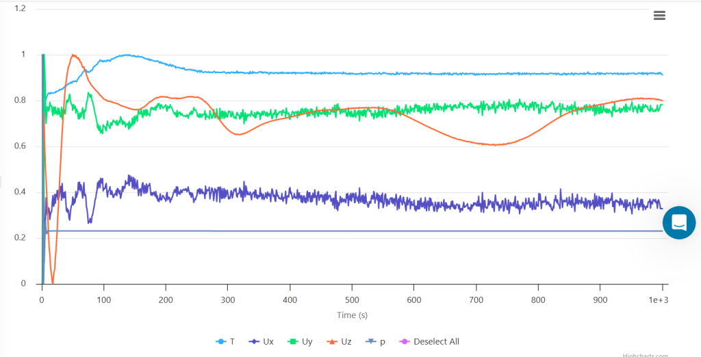
In the third image, multiple lines (representing temperature, velocity components, and possibly pressure) are monitored at the outlet.
- Temperature (T):
- Starts at some initial value or a transient state, then converges to a stable outlet temperature.
- The difference between the hot-side inlet and the outlet temperature is a direct measure of how much cooling occurred.
- Velocity Components (Ux, Uy, Uz):
- These curves also start with higher oscillations but eventually flatten out.
- Minor fluctuations may remain if there is any swirl or complex recirculation near the outlet.
- Pressure (P):
- Typically set to a reference at the outlet, though small variations can occur due to local flow dynamics.
When these lines become relatively flat and remain within a narrow band, it confirms that your solution has reached a steady or quasi-steady state.