TUGAS AKHIR KOMPUTASI TEKNIK- Febryan Andhika Saputra (2406375522)

A. Project Title

Development of an AI Assistant for Generating Python Code to Analyze One Dimensional Temperature Distribution in Plate Fin Heat Conduction Using Analytical and Finite Difference Methods

B.Author Complete Name

Febryan Andhika Saputra

C. Affiliation

Department of Mechanical Engineering, Faculty of Engineering, Universitas Indonesia.

D. Abstract

This project develops an AI assistant using the AI DAI5 with DAI5 Framework, to evaluate the capability of an AI assistant in automatically generating Python code to solve one dimensional steady state heat conduction problems using both analytical and numerical methods approaches. The physical model is based purely on conduction, with no convection or heat generation, and assumes constant thermal conductivity along the plate. The analytical solution is derived directly from the 1D steady-state conduction equation, resulting in a linear temperature distribution between two fixed boundary temperatures. The numerical solution is computed using the Finite Difference Method (FDM), where the spatial domain is discretized into uniform nodes and the temperature at interior points is solved iteratively until convergence criteria are met. The AI assistant follows a structured algorithm based on receiving input parameters, generating the analytical solution, constructing an FDM grid, performing iterative updates, checking convergence, storing numerical results, and producing a comparison table with error values. It also automatically generates line plots showing analytical and numerical temperature profiles. Results indicate that the numerical FDM solution converges closely to the analytical solution when appropriate node spacing and tolerance values are used. This demonstrates the ability of the AI system to support engineering computation tasks by automating code generation, numerical solving, and visualization in heat conduction analysis.

E. Author Declaration

1. Deep Awareness (of) I

In carrying out this project, I acknowledge that the natural laws governing heat conduction such as Fourier’s law and the behavior of thermal equilibrium is part of the order established by the Creator. This awareness reminds me to approach the development of the AI assistant with humility, responsibility, and honesty. I recognize that the ability to understand physics, mathematics, and computation is a trust that must be used ethically and beneficially.

2. Intention of the Project Activity

The intention of this project is to create an AI assistant capable of generating Python code that solves one-dimensional steady-state heat conduction along the plate fin problems using both analytical and Numerical using Finite Difference Methods. This project aims to support students, researchers, and practitioners by simplifying computation, improving accuracy, and enhancing conceptual understanding. The objectives are grounded in a desire to develop useful tools, promote transparent scientific computation, and contribute positively to engineering education and practice.

F. Introduction

Heat conduction is one of the fundamental modes of heat transfer and plays an essential role in engineering applications such as thermal insulation, heat exchangers, metal casting, electronic cooling, and structural materials exposed to thermal gradients. In many practical situations, heat transfer occurs predominantly in one direction, allowing a one-dimensional conduction model to be used effectively.

For a solid plate (or bar) under steady-state conditions with constant thermal conductivity and no internal heat generation, the governing equation simplifies to:

This differential equation leads to a linear temperature distribution between two fixed boundary temperatures. While the analytical solution is straightforward, numerical methods such as the Finite Difference Method (FDM) are widely applied because they can handle more complex scenarios, different boundary conditions, and discretization-based approximations for higher-dimensional cases.

To support students and engineers in understanding conduction more intuitively, this project develops an AI assistant that can automatically generate Python code to compute the temperature distribution analytically and numerically, compare both solutions, form a table of results, and generate corresponding plots. The AI follows a structured algorithm ensuring that the computation is systematic, accurate, and easy to reproduce.

1. Initial Thinking (About the Problem)

Before implementing the AI assistant, it is necessary to clearly define the problem structure:

The objective is to model pure 1D steady-state conduction, without convection, radiation, or heat generation.
The boundary temperatures at the left and right ends of the plate are known (Dirichlet boundary conditions).
The analytical solution must be generated from the simplified conduction equation and boundary values.
The numerical solution must follow the Finite Difference Method, by discretizing the plate into uniform nodes and iteratively updating interior temperatures until convergence.
The AI must integrate the entire sequence: input reading, analytical computation, grid creation, FDM computation, convergence checking, data storage, error calculation, and automatic plot generation.

This early conceptualization ensures that the AI assistant is coherent, aligned with physical principles, and capable of producing reliable and interpretable results.

G.Methods & Procedures

1.Idealization

To formulate the physical problem in a solvable mathematical form, several ideal assumptions are applied:

Heat transfer occurs only by pure conduction, with no convection and no radiation.
The system is in steady-state, meaning the temperature does not vary with time.
Thermal conductivity is constant throughout the plate.
No internal heat generation is present within the domain.
Heat transfer is one-dimensional along the x-axis.
Boundary temperatures at the left and right ends are known (Dirichlet boundary conditions).
The geometry requires only the plate length L; width and thickness are relevant only for heat-rate calculations.

Under these assumptions, the governing differential equation reduces to:

which yields a linear analytical temperature distribution.

2.Instruction Set

This section follows the sequence of the provided process flowchart below and describes how the AI assistant generates the solution.

a. Input of Physical Parameters

The AI receives the following physical inputs:

Plate length L
Thermal conductivity k
Left boundary temperature Tleft
Right boundary temperature Tright

Width and thickness may be included if heat flux or heat rate is required.

b. Input of Numerical Parameters

The AI accepts:

Number of nodes (N)
Convergence tolerance (ϵ)
Maximum number of iterations (max_iter)

c. Analytical Solution

Using the simplified 1D conduction equation, the analytical temperature profile is calculated as:

the heat lux is computed as:

d. Discretization

The AI construct the numerical grid:

Nodes are distributed uniformly from x=0 to x=L.
Initial guesses for interior temperatures are generated (e.g., zeros or linier interpolation).

e. Numerical Method Finite Difference Method (FDM)

The AI uses the standard steady-state 1 finite-difference formulation for interior nodes:

The numerical solution is obtained using Gauss-Seidel iteration,wher updated values are used immediately (in place) as the sweep progresses.
The update formulas applied at each iteration step is:

After each full sweep over all interior nodes, the AI computes the maximum temperature change:

Iteration continue until Δmax falls below the user defines tolerance or until the maximum iteration limit is reached

f. Convergence Check

The algorithm evaluates whether:

Convergence is achieved store the final temperature distribution
Convergence is not achieved but iterations reach the limit store result and flag as “not fully converged”.

g. Storage Of Numerical Result

The AI records:

Node Coordinates
Final numerical temperatures
Number of Iterations
Convergence Status
Associated Errors metrics

h. Generation of Comparison Table

A structured table is produces containing:

I Node x (m)I Analytical Temperature (Cº) I Numerical Temperature (Cº)I Error (%) I

with error computed as:

i. Generation Of Plots

The AI automatically generates:

A line plot comparing analytical and numerical temperature distributions
(Optional) an iteration history plot to show numerical convergence behavior

These outputs complete the computation sequence described by the flowchart process.

H. Result and Discussion

Based on the implementation result, the AI assistant successfully responded to user prompts related to fundamental heat transfer concept, one dimensional heat conduction, numerical method, and Phyton code generation. The AI demonstrated the ability to explain heat transfer conceptually, distinguish between thermodynamics and heat transfer , and correctly identify conduction as the sole heat transfer mode analyzed in this study
In the computational stage, the AI Assistant automatically generated a complete Python program to analyze the steady-state one-dimensional heat conduction of an aluminum plate fin with fixed temperature boundary conditions at both ends. The physical model strictly assumes one-dimensional conduction, steady-state conditions, constant thermal conductivity, and the absence of convection, radiation, and internal heat generation. Under these assumptions, the analytical solution produced by the AI is a linear temperature distribution along the plate length, which is consistent with the exact solution of the one-dimensional heat conduction equation.
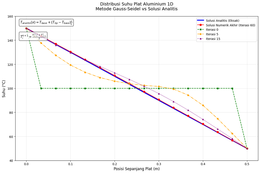
The numerical solution was obtained using the Finite Difference Method (FDM), with the resulting system of algebraic equations solved iteratively using the Gauss–Seidel method. The AI Assistant correctly implemented domain discretization, initial temperature guessing, iterative updating of nodal temperatures, and convergence checking based on a predefined tolerance value (e=10^-4) The numerical solution converged smoothly to the analytical solution, achieving an average relative error of 0.4023%, which indicates a high level of numerical accuracy for the selected discretization and convergence criteria.

The generated comparison table presents the analytical and numerical temperature values at each node along the plate, along with their relative errors. The graphical visualization further confirms the accuracy of the numerical approach, as the final numerical temperature profile closely overlaps with the analytical solution. Additionally, intermediate iteration curves illustrate the convergence behavior of the Gauss–Seidel method, providing clear insight into the iterative solution process.

I. Conclusion, Closing Remarks, and Recommendations
a) Conclusion
This study successfully developed an AI Assistant capable of automatically generating Python code for analyzing one-dimensional steady-state heat conduction using both analytical and Finite Difference Method approaches. The AI Assistant demonstrated the ability to explain theoretical concepts, formulate numerical models, implement iterative solvers, and present results in the form of tables and graphical comparisons. The close agreement between analytical and numerical solutions confirms the correctness and reliability of the generated code.

b) Closing Remarks
The integration of AI into heat transfer analysis offers significant potential for improving both computational efficiency and learning effectiveness. By following the DAI5 framework, this project emphasizes not only numerical accuracy but also structured thinking, physical awareness, and clarity of algorithmic instruction. As a result, the AI Assistant serves as both a computational tool and an educational aid in heat conduction analysis.
c) Recommendations
Future work may extend the AI Assistant to transient heat conduction problems, two-dimensional conduction models, or cases involving spatially varying material properties. Additional numerical techniques and error analysis strategies may also be incorporated to further enhance the robustness and versatility of the system.

J. Acknowledgments
The author gratefully acknowledges the academic literature and educational resources that form the foundation of heat transfer theory and numerical methods. Appreciation is also extended to the DAI5 framework and AI DAI5 created by Prof. Ahmad Indra Siswantara, PhD at Universitas Indonesia, which guided the systematic and reflective development of the AI Assistant.

K. References

Holman J.P, Heat Transfer Tenth Edition
Frank P Incropera, Introduction to Heat Transfer Sixth Edition
Jaan Kiusalaas, Numerical Methods in Engineering with Python 3
Prof. Ir. Ahmad Indra Siswantara, Ph.D, DAI5 “Deep Awareness of I”

L. Appendices
Appendices are provided to support transparency, reproducibility, and technical completeness of the AI-assisted heat conduction analysis. The materials included in this section contain detailed algorithmic steps, mathematical formulations, and computational outputs that are not presented in the main body of the report

APPENDIX A: Governing Equation and Boundary Conditions

This appendix presents the mathematical model used in the analysis.

The governing equation for one-dimensional steady-state heat conduction without internal heat generation is:

Boundary conditions applied in this study are of Dirichlet type:

Under these conditions, the analytical solution is:

APPENDIX B: Finite Difference Method Discretization

The spatial domain is discretized into N equally spaced nodes with spacing:

The second-order central difference approximation of the second derivative yields the nodal equation for interior nodes:

which can be rearranged as:

APPENDIX C: Iterative Solution Using Gauss–Seidel Method

To solve the system of algebraic equations resulting from the Finite Difference Method, the Gauss–Seidel iterative scheme is applied.
The Update equation for iteration k+1 is:

The convergence criterion is defined as:

where=10^-4 is the convergence tolerance.

APPENDIX D: Algorithm Flowchart Description

The flowchart outlines the complete computational workflow, ensuring consistency, reproducibility, and alignment with the Finite Difference Method (FDM) and Gauss–Seidel iterative scheme. The steps are described as follows:

1.Start
Initialize the computational process.
2. Input Physical and Numerical Parameters
Define the plate length, cross-sectional dimensions, thermal conductivity, boundary temperatures, number of nodes, convergence tolerance (ε), and maximum number of iterations.
3. Define Governing Equation and Boundary Conditions
Apply the one-dimensional steady-state heat conduction equation without internal heat generation and specify Dirichlet boundary conditions at both ends of the plate.
4. Discretize Spatial Domain
Divide the plate length into equally spaced nodes using the Finite Difference Method.
5. Initialize Temperature Field
Assign an initial temperature guess for all interior nodes while enforcing the boundary temperatures at the first and last nodes.
6. Iterative Solution Using Gauss–Seidel Method
Update the temperature of each interior node sequentially using the Gauss–Seidel formulation based on neighboring node values.
7. Check Convergence Criterion
Evaluate the maximum absolute difference between successive iterations. If the difference is smaller than the prescribed tolerance, convergence is achieved.
8. Iteration Control
If convergence is not satisfied and the maximum number of iterations has not been reached, return to the iteration step.
9. Compute Analytical Solution
Calculate the analytical temperature distribution based on the closed-form solution for one-dimensional steady-state conduction.
10. Error Evaluation
Compute the relative error between numerical and analytical temperature values at each node.
11. Store Results
Save numerical temperatures, analytical temperatures, iteration history, and error data.
12. Generate Output Tables
Present a comparison table of numerical and analytical solutions along with relative errors.
13. Generate Graphical Visualization
Plot the temperature distribution along the plate length, including analytical solution, final numerical solution, and selected intermediate iterations to illustrate convergence behavior.
14. End
Terminate the computational process.

This flowchart ensures that the AI-generated Python code follows a logically structured and physically consistent solution procedure for one-dimensional heat conduction analysis.

APPENDIX E: AI Phyton Code Generated

import numpy as np
import matplotlib.pyplot as plt

# ======================================================
# DATA INPUT KASUS - PLAT ALUMINIUM
# ======================================================
L_batang = 0.50        # Panjang batang (meter) - 500 mm
W_batang = 0.10        # Lebar batang (meter) - 100 mm
t_batang = 0.010       # Tebal batang (meter) - 10 mm
k_batang = 237.0       # Konduktivitas termal aluminium (W/m·K)
T_base_batang = 150.0  # Suhu di x=0 (°C)
T_tip_batang = 50.0    # Suhu di x=L (°C)
N_nodes = 16           # Jumlah node
epsilon_toleransi = 1e-4 # Kriteria konvergensi
max_iterasi = 60       # Batas maksimum iterasi
# ======================================================

## Fungsi Solusi Analitis dan Laju Panas
def solusi_analitis_dan_panas(x_pos, L, T_base, T_tip, k, W, t):
    """
    Menghitung distribusi suhu analitis (linier) dan laju panas konduksi (q).
    Persamaan: T_analitis(x) = T_base + (T_tip - T_base) * (x/L)
    """
    T_analitis = T_base + (T_tip - T_base) * (x_pos / L)
    Area = W * t
    gradien_T = (T_tip - T_base) / L
    q = -k * Area * gradien_T  # Fourier's Law
    return T_analitis, q

## Fungsi Solusi Numerik Gauss-Seidel
def gauss_seidel_solver(x_pos, T_initial, T_base, T_tip, tol, max_iter):
    """
    Memecahkan konduksi panas 1D menggunakan metode Gauss-Seidel.
    Persamaan nodal: T_i^{k+1} = (T_{i-1}^{k+1} + T_{i+1}^k)/2
    """
    N = len(T_initial)
    T_k = T_initial.copy()

    # Dictionary untuk menyimpan riwayat suhu pada iterasi tertentu
    riwayat_iterasi = {}
    iterasi_simpan = {0, 5, 15}

    for k in range(1, max_iter + 1):
        T_k_plus_1 = T_k.copy()

        # Simpan array suhu pada iterasi kunci
        if k - 1 in iterasi_simpan:
            riwayat_iterasi[f"Iterasi {k-1}"] = T_k.copy()

        # Iterasi Gauss-Seidel untuk node interior (i=1 hingga N-2)
        for i in range(1, N - 1):
            T_k_plus_1[i] = 0.5 * (T_k_plus_1[i-1] + T_k[i+1])

        # Kriteria Konvergensi
        diff = np.max(np.abs(T_k_plus_1 - T_k))
        T_k = T_k_plus_1

        if diff < tol:
            print(f"Konvergensi tercapai setelah {k} iterasi. Error: {diff:.6e}")
            break

    # Simpan iterasi akhir jika belum tersimpan
    if k not in iterasi_simpan:
        riwayat_iterasi[f"Iterasi {k}"] = T_k.copy()

    return T_k, riwayat_iterasi, k

# ======================================================
# EKSEKUSI PROGRAM
# ======================================================

# 1. Inisialisasi Posisi Node dan Tebakan Awal
x_nodes = np.linspace(0, L_batang, N_nodes)
T_avg = (T_base_batang + T_tip_batang) / 2  # Tebakan rata-rata
T_initial = np.full(N_nodes, T_avg)
T_initial[0] = T_base_batang  # Kondisi batas x=0
T_initial[-1] = T_tip_batang  # Kondisi batas x=L

# 2. Hitung Solusi Analitis
T_analitis_sol, q_panas = solusi_analitis_dan_panas(
    x_nodes, L_batang, T_base_batang, T_tip_batang, k_batang, W_batang, t_batang
)

# 3. Hitung Solusi Numerik Gauss-Seidel
T_numerik_akhir, riwayat_solusi, iter_akhir = gauss_seidel_solver(
    x_nodes, T_initial, T_base_batang, T_tip_batang, epsilon_toleransi, max_iterasi
)

# ======================================================
# OUTPUT WAJIB
# ======================================================

print("\n" + "="*75)
print("🌡️ ANALISIS KONDUKSI PANAS 1D - PLAT ALUMINIUM")
print("="*75)

## 1. Informasi Material dan Laju Panas
print(f"\n1. INFORMASI MATERIAL:")
print(f"- Panjang plat: {L_batang*1000:.1f} mm")
print(f"- Lebar plat: {W_batang*1000:.1f} mm")
print(f"- Tebal plat: {t_batang*1000:.1f} mm")
print(f"- Konduktivitas termal: {k_batang} W/m·K")
print(f"- Laju Panas Konduksi (q): {abs(q_panas):.2f} Watt")

## 2. Tabel Perbandingan
error_relatif = np.abs(T_numerik_akhir - T_analitis_sol) / T_analitis_sol * 100

print(f"\n2. TABEL PERBANDINGAN SUHU (Konvergensi pada iterasi {iter_akhir}):")
print("-"*75)
print(f"{'Posisi x [m]':<12} | {'T_analitis [°C]':<15} | {'T_numerik [°C]':<15} | {'Error (%)':<10}")
print("-"*75)

for i, (x, Ta, Tn, Err) in enumerate(zip(x_nodes, T_analitis_sol, T_numerik_akhir, error_relatif)):
    print(f"{x:<12.3f} | {Ta:<15.2f} | {Tn:<15.2f} | {Err:<10.4f}")

print("-"*75)
print(f"Error relatif rata-rata: {np.mean(error_relatif):.4f}%")

## 3. Grafik Visualisasi
plt.figure(figsize=(12, 8))

# Kurva solusi analitis
plt.plot(x_nodes, T_analitis_sol, 'b-', linewidth=3, label='Solusi Analitis (Eksak)')

# Kurva solusi numerik akhir
plt.plot(x_nodes, T_numerik_akhir, 'ro-', markersize=6, label=f'Solusi Numerik Akhir (Iterasi {iter_akhir})')

# Kurva iterasi awal untuk menunjukkan konvergensi
colors = ['g', 'orange', 'purple']
markers = ['s', 'D', '^']
linestyles = ['--', '-.', ':']

for i, (label, T_hist) in enumerate(list(riwayat_solusi.items())[:3]):
    plt.plot(x_nodes, T_hist, color=colors[i], marker=markers[i],
             linestyle=linestyles[i], linewidth=1.5, markersize=4, label=label)

plt.title('Distribusi Suhu Plat Aluminium 1D\nMetode Gauss-Seidel vs Solusi Analitis', fontsize=14, pad=20)
plt.xlabel('Posisi Sepanjang Plat (m)', fontsize=12)
plt.ylabel('Suhu (°C)', fontsize=12)
plt.grid(True, alpha=0.3)
plt.legend(fontsize=10)
plt.ylim(T_tip_batang-10, T_base_batang+10)

# Anotasi persamaan
plt.text(0.02, 0.95, r'$T_{analitis}(x) = T_{base} + (T_{tip} - T_{base})\frac{x}{L}$',
         transform=plt.gca().transAxes, fontsize=11, bbox=dict(boxstyle="round,pad=0.3", fc="white", alpha=0.8))
plt.text(0.02, 0.85, r'$T_i^{k+1} = \frac{T_{i-1}^{k+1} + T_{i+1}^k}{2}$',
         transform=plt.gca().transAxes, fontsize=11, bbox=dict(boxstyle="round,pad=0.3", fc="white", alpha=0.8))

plt.tight_layout()
plt.show()

print(f"\n3. GRAFIK BERHASIL DIGENERATE!")
print("="*75)

APPENDIX F: Numerical Results and Error Analysis