Zahran Nadhif Afdallah Malik-2306155451
Physical-Informed Neural Networks (PINNs) are a type of neural network that incorporates physical laws or constraints into their architecture during training. This approach allows PINNs to solve complex problems involving real-world systems more effectively by leveraging known physical principles.
Here’s an overview of PINNs:
- Neural Networks and Deep Learning: PINNs build upon traditional neural networks, which are designed for pattern recognition and data processing. However, PINNs extend these models by integrating physical constraints or equations.
- Partial Differential Equations (PDEs): PINNs incorporate PDEs, which describe how physical systems change over space and time. These equations are often derived from fundamental laws like conservation of mass, energy, momentum, or force.
- Loss Functions: PINNs use loss functions that include terms enforcing the physical constraints. This ensures that the neural network’s predictions satisfy these physical laws, improving accuracy and physical consistency.
- Training Process: During training, PINNs are optimized using gradient descent, which minimizes a combination of prediction error (training loss) and constraint satisfaction (regularization loss).
- Applications: PINNs are particularly useful for solving forward and inverse problems in domains such as fluid dynamics, materials science, climate modeling, and more.
In summary, PINNs combine the power of neural networks with physical constraints, making them effective for real-world applications where understanding the underlying physics is crucial.
This time i will try to simulate a 1d heat conduction using PINN approach, here is the case:
heat was given to a 1m stainless steel block. the temperature at one end is T0=100 celcius and the other end is 0 celcius, simulate the heat conduction using PINN approach:
DAI5 Framework
- Awareness: Physical-Informed Neural Networks (PINNs) are a type of artificial neural network that integrates physical laws and constraints into the learning process to enhance their performance in real-world applications. Unlike traditional neural networks, which learn patterns from data alone, PINNs incorporate known equations or principles from physics or other domains. This integration ensures that the network’s predictions not only fit the training data but also adhere to the underlying physical laws, making them more accurate and reliable for scientific and engineering tasks. During training, PINNs use a loss function that includes terms enforcing physical constraints. For example, if modeling fluid flow, the network would ensure that conservation laws like mass or momentum are satisfied, improving its ability to generalize and predict behavior accurately. This approach is particularly valuable in fields such as climate modeling, material science, and engineering design, where understanding and respecting physical principles is crucial.
- Intention: simulating a 1d heat conduction using PINN approach
- Initial thingking
1d heat conduction formula
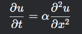
where t is time distribution, u is temperature distribution, and a is thermal conductivity
4. Idealization
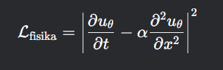
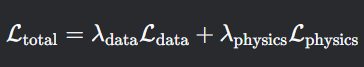
- Physical loss
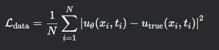
- loss data
- total loss
and here are some idealization on the stainless steel block
- the length is right 1m, no error
- the thermal conductivity is right 16,2 wm/K
- the temperature is right T0=100 celcius at one end and T1=0 celcius at the other end
- steady state condition on the stainless steel block
5. Instruction set
next, i tried to simulate the heat conduction through python programming, here is the code:
# Import Libraries
import torch
import torch.nn as nn
import numpy as np
import matplotlib.pyplot as plt
# Define PINN Class
class PINN(nn.Module):
def __init__(self):
super(PINN, self).__init__()
self.net = nn.Sequential(
nn.Linear(1, 25), # Mengubah jumlah neuron pada layer pertama
nn.Tanh(),
nn.Linear(25, 25), # Mengubah jumlah neuron pada hidden layer
nn.Tanh(),
nn.Linear(25, 1)
)
def forward(self, x):
return self.net(x)
# Compute Loss Function
def compute_loss(model, x, T0, T1):
x = x.requires_grad_(True)
T = model(x)
# Compute derivatives
dT_dx = torch.autograd.grad(T, x, grad_outputs=torch.ones_like(T), create_graph=True)[0]
d2T_dx2 = torch.autograd.grad(dT_dx, x, grad_outputs=torch.ones_like(dT_dx), create_graph=True)[0]
# Physics loss
physics_loss = torch.mean(d2T_dx2**2)
# Boundary conditions
T_left = model(torch.tensor([[0.0]]))
T_right = model(torch.tensor([[1.0]]))
bc_loss = (T_left - T0)**2 + (T_right - T1)**2
return physics_loss + bc_loss
# Train PINN Function
def train_pinn(T0, T1, epochs=1000):
model = PINN()
optimizer = torch.optim.Adam(model.parameters(), lr=0.0099) # Mengubah learning rate
x = torch.linspace(0, 1, 120).reshape(-1, 1) # Menambah jumlah titik diskritisasi
for epoch in range(epochs):
optimizer.zero_grad()
loss = compute_loss(model, x, T0, T1)
loss.backward()
optimizer.step()
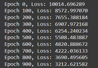
if epoch % 100 == 0:
print(f"Epoch {epoch}, Loss: {loss.item():.6f}")
return model
# Plot Result Function
def plot_results(model, T0, T1):
x = torch.linspace(0, 1, 120).reshape(-1, 1)
with torch.no_grad():
T_pred = model(x).numpy()
x = x.numpy()
T_analytical = T0 + (T1 - T0) * x
plt.figure(figsize=(8, 6))
plt.plot(x, T_pred, label="PINN Solution", linewidth=2)
plt.plot(x, T_analytical, "--", label="Analytical Solution", linewidth=2)
plt.xlabel("x")
plt.ylabel("Temperature")
plt.title("1D Steady-State Heat Conduction")
plt.legend()
plt.grid(True)
# Simpan grafik sebagai file jika tidak ada display
plt.savefig("heat_conduction_result_updated.png")
print("Grafik telah disimpan sebagai 'heat_conduction_result_updated.png'")
# Main Execution
if __name__ == "__main__":
# Parameter default
T0 = 100.0 # Suhu di x=0
T1 = 0.0 # Suhu di x=1
epochs = 1000
# Latih model dan tampilkan hasil
model = train_pinn(T0, T1, epochs)
plot_results(model, T0, T1)and here are the results: