ccitonline.com

Curve Fitting

Curve Fitting Visualization

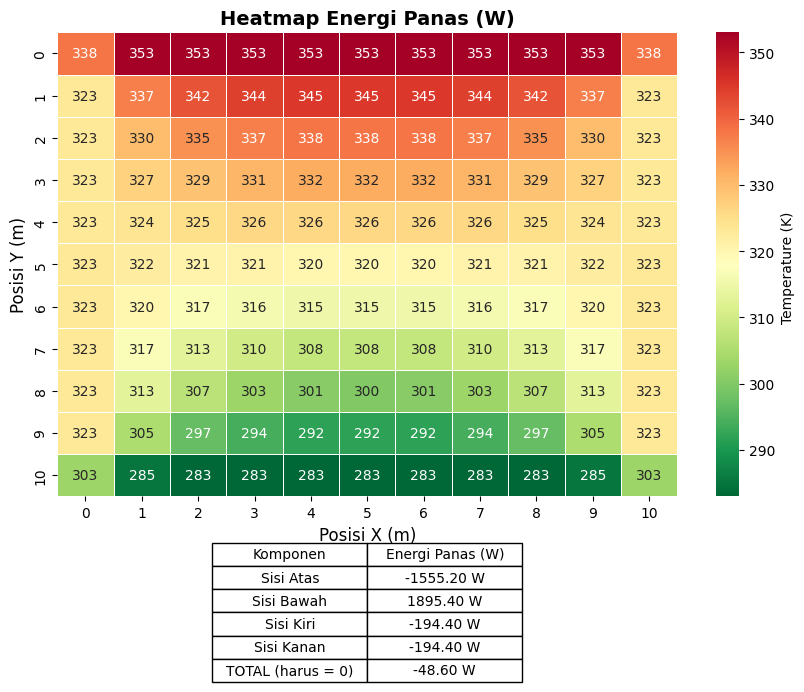
Sumbu X: Posisi (m), Sumbu Y: Temperatur (K)

Heatmap

import numpy as np
import matplotlib.pyplot as plt
import seaborn as sns

# Konduktivitas termal (W/mK)
k = 16.2

# Data temperatur dari 2dtemp11 hingga 2dtemp1 (dibalik urutannya)
temp_data = np.array([
    [338, 353, 353, 353, 353, 353, 353, 353, 353, 353, 338],
    [323, 337, 342, 344, 345, 345, 345, 344, 342, 337, 323],
    [323, 330, 335, 337, 338, 338, 338, 337, 335, 330, 323],
    [323, 327, 329, 331, 332, 332, 332, 331, 329, 327, 323],
    [323, 324, 325, 326, 326, 326, 326, 326, 325, 324, 323],
    [323, 322, 321, 321, 320, 320, 320, 321, 321, 322, 323],
    [323, 320, 317, 316, 315, 315, 315, 316, 317, 320, 323],
    [323, 317, 313, 310, 308, 308, 308, 310, 313, 317, 323],
    [323, 313, 307, 303, 301, 300, 301, 303, 307, 313, 323],
    [323, 305, 297, 294, 292, 292, 292, 294, 297, 305, 323],
    [303, 285, 283, 283, 283, 283, 283, 283, 283, 285, 303]
])

# Menghitung gradien suhu untuk menghitung energi panas (konduksi Fourier)
dx = 0.1  # Interval grid (m)
dTdx_top = (temp_data[0, 1:-1] - temp_data[1, 1:-1]) / dx
dTdx_bottom = (temp_data[-1, 1:-1] - temp_data[-2, 1:-1]) / dx
dTdy_left = (temp_data[1:-1, 0] - temp_data[1:-1, 1]) / dx
dTdy_right = (temp_data[1:-1, -1] - temp_data[1:-1, -2]) / dx

# Menghitung energi panas di tiap sisi
Q_top = -k * np.sum(dTdx_top) * dx
Q_bottom = -k * np.sum(dTdx_bottom) * dx
Q_left = -k * np.sum(dTdy_left) * dx
Q_right = -k * np.sum(dTdy_right) * dx

# Total energi panas
Q_total = Q_top + Q_bottom + Q_left + Q_right

# Plot heatmap
fig, ax = plt.subplots(figsize=(10, 8))
cmap = sns.color_palette("RdYlGn_r", as_cmap=True)
sns.heatmap(temp_data, annot=True, fmt=".0f", cmap=cmap, linewidths=0.5, ax=ax, cbar_kws={'label': 'Temperature (K) '})
ax.set_title("Heatmap Energi Panas (W)", fontsize=14, fontweight='bold')
ax.set_xlabel("Posisi X (m)", fontsize=12)
ax.set_ylabel("Posisi Y (m)", fontsize=12)

# Menampilkan informasi energi panas dalam plot
table_data = [["Sisi Atas", f"{Q_top:.2f} W"],
              ["Sisi Bawah", f"{Q_bottom:.2f} W"],
              ["Sisi Kiri", f"{Q_left:.2f} W"],
              ["Sisi Kanan", f"{Q_right:.2f} W"],
              ["TOTAL (harus = 0)", f"{Q_total:.2f} W"]]

table = plt.table(cellText=table_data, colLabels=["Komponen", "Energi Panas (W)"], cellLoc='center', loc='bottom', bbox=[0.25, -0.4, 0.5, 0.3])
table.auto_set_font_size(False)
table.set_fontsize(10)

plt.subplots_adjust(bottom=0.3)
plt.show()